Usage

Quick start guide to use hierarchical linear regression using HLR package.

Fetch example data

Let’s first fetch some data and initiate the HLR object. We’ll use the penguins dataset from seaborn for our example.

import seaborn as sns
import pandas as pd

# Load the example penguins dataset
df = sns.load_dataset('penguins')
df.dropna(inplace=True)
df = df[['bill_length_mm', 'bill_depth_mm', 'flipper_length_mm', 'body_mass_g']]

Initialize HLR & generate summary report

from HLR import HierarchicalLinearRegression

# Define the independent variables for each model level
ivs_dict = {
     1: ['bill_length_mm'],
     2: ['bill_length_mm', 'bill_depth_mm'],
     3: ['bill_length_mm', 'bill_depth_mm', 'flipper_length_mm']
}

# Define the dependent variable
dv = 'body_mass_g'

# Initialize the HierarchicalLinearRegression class
hlr = HierarchicalLinearRegression(df, ivs_dict, dv)
hlr.summary()

Output:

Model Level	Predictors	N (observations)	DF (residuals)	DF (model)	R-squared	F-value	P-value (F)	SSR	SSTO	MSE (model)	MSE (residuals)	MSE (total)	Beta coefs	P-values (beta coefs)	Std Beta coefs	Partial correlations	Semi-partial correlations	Unique variance %	R-squared change	F-value change	P-value (F-value change)
1	[bill_length_mm]	333.0	331.0	1.0	0.35	176.24	0.0	140467132.89	215259665.92	74792533.03	424372.00	648372.49	{'const': 388.85, 'bill_length_mm': 86.79}	{'const': 0.18, 'bill_length_mm': 0.0}	{'bill_length_mm': 0.59}	{'bill_length_mm': 0.59}	{'bill_length_mm': 0.59}	{'bill_length_mm': 34.75}	NaN	NaN	NaN
2	[bill_length_mm, bill_depth_mm]	333.0	330.0	2.0	0.47	144.84	0.0	114633408.59	215259665.92	50313128.67	347373.97	648372.49	{'const': 3413.45, 'bill_length_mm': 74.81, 'bill_depth_mm': -145.51}	{'const': 0.0, 'bill_length_mm': 0.0, 'bill_depth_mm': 0.0}	{'bill_length_mm': 0.51, 'bill_depth_mm': -0.36}	{'bill_length_mm': 0.56, 'bill_depth_mm': -0.43}	{'bill_length_mm': 0.49, 'bill_depth_mm': -0.35}	{'bill_length_mm': 24.47, 'bill_depth_mm': 12.0}	0.12	74.37	0.0
3	[bill_length_mm, bill_depth_mm, flipper_length_mm]	333.0	329.0	3.0	0.76	354.90	0.0	50814911.80	215259665.92	54814918.04	154452.62	648372.49	{'const': -6445.48, 'bill_length_mm': 3.29, 'bill_depth_mm': 17.84, 'flipper_length_mm': 50.76}	{'const': 0.0, 'bill_length_mm': 0.54, 'bill_depth_mm': 0.2, 'flipper_length_mm': 0.0}	{'bill_length_mm': 0.02, 'bill_depth_mm': 0.04, 'flipper_length_mm': 0.88}	{'bill_length_mm': 0.03, 'bill_depth_mm': 0.07, 'flipper_length_mm': 0.75}	{'bill_length_mm': 0.02, 'bill_depth_mm': 0.03, 'flipper_length_mm': 0.54}	{'bill_length_mm': 0.03, 'bill_depth_mm': 0.12, 'flipper_length_mm': 29.65}	0.30	413.19	0.0

Run diagnostics for testing assumptions

diagnostics_dict = hlr.diagnostics(verbose=True)

Output:

Model Level 1 Diagnostics:
Independence of residuals (Durbin-Watson test):
DW stat: 0.8450671190941991
Passed: False
Linearity (Pearson r):
bill_length_mm: {'Pearson r': 0.5894511101769488, 'p-value': 1.5386135144860176e-32, 'Passed': True}
Linearity (Rainbow test):
Rainbow Stat: 0.845825915500362
p-value: 0.8589217163587981
Passed: True
Homoscedasticity (Breusch-Pagan test):
Lagrange Stat: 76.51043993569607
p-value: 2.1905189444330245e-18
Passed: False
Homoscedasticity (Goldfeld-Quandt test):
F-Stat: 3.298385120028286
p-value: 5.1841847326260096e-14
Passed: False
Multicollinearity (pairwise correlations):
Correlations: {}
Passed: True
Multicollinearity (Variance Inflation Factors):
VIFs: {}
Passed: True
Outliers (extreme standardized residuals):
Indices: []
Passed: True
Outliers (high Cooks distance):
Indices: []
Passed: True
Normality (mean of residuals):
Mean: -2.403469482162693e-13
Passed: True
Normality (Shapiro-Wilk test):
SW Stat: 0.9912192354166119
p-value: 0.04492289320888261
Passed: False

Model Level 2 Diagnostics:
...

Plotting options for all model levels

fig = hlr.plot_studentized_residuals_vs_fitted()

Output:

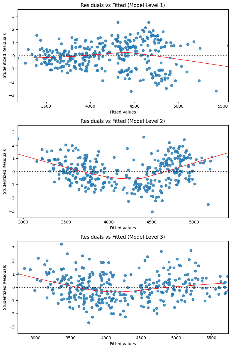
fig = hlr.plot_qq_residuals()

Output:

fig = hlr.plot_influence()

Output:

fig = hlr.plot_std_residuals()

Output:

fig = hlr.plot_histogram_std_residuals()

Output:

fig_list = hlr.plot_partial_regression()

Output:

(the fig_list contains a fig for each Model Level; only Model Level 1 displayed (i.e., fig_list[0]))